OpenCV or Open Computer Vision Library is one of the widely accepted opensource Library for image processing and computer vision applications. OpenCV supports Python, this feature makes OpenCV as the default choice for Deep learning application for computer vision. This blog post shows how basic image processing operations can be carried out using Python OpenCV package.
- Loading Image data and extract color channels.
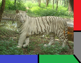
The Code snippet given below shows reading the image file and working on pixel data. The original image used for this example is shown below. This is a tiger image which to which I have added Red, Green, and Blue color border on the left side and bottom.
import numpy as np
import cv2
print (cv2.__version__)

img_data =cv2.imread ("C:/Users/admin/c2plabs/tiger.png",1)
print (img_data.shape)
cv2.imshow ("Original",img_data)
cv2.moveWindow ("Original",0,0)

b = img_data [:,:,0]

g = img_data [:,:,1]

r = img_data [:,:,2]


bgr_all = np.concatenate ((b,g,r),axis=1)

cv2.imshow ("split",bgr_all)
cv2.moveWindow ("split",0,550)
cv2.waitKey(0)
cv2.destroyAllWindows()
Let’s see how above code snippet executes. The first three lines related to importing numpy and OpenCV libraries and printing the version of OpenCV library. If OpenCV is not properly installed on your working environment error will be thrown.
At line no 5 we are reading the image data using cv2.imread function, this takes two arguments file path and read flag. This flag value can be cv2.IMREAD_COLOR (value 1) or cv2.IMREAD_GRAYSCALE (value 0) or cv2.IMREAD_UNCHANGED (-1). Here we are using ‘1’ to read color data.
The return value of cv2.imread function is a numpy array of type ‘ndarray’. This is a multidimensional array that stores pixel data of the image. Line 6 prints img_data.shape which gives the dimension of the image.
The output of line 6 is (215, 275, 3). Here 215 is the height of image and 275 is the width of the image and 3 is the color depth of the image (B, G, R). Code at line 7,8 is used to display the image. Function cv2.imshow display image in a new window with window name “Original”. The function cv2.moveWindow (“Original”,0,0) moves the displayed window to top left of the desktop.
In lines 10,12 and 14 we are extracting blue pixel data, green pixel data, and red pixel data respectively. Here nupmy array slicing operation is used to get the required information. This can be achieved cv2.slipt function also.
b = img_data [:,:,0] # This line read all the rows, columns from img_data at depth 0.
g = img_data [:,:,1] # This line read all the rows, columns from img_data at depth 1.
r= img_data [:,:,2] # This line read all the rows, columns from img_data at depth 2.
Note: b,g,r = cv2.split (img_data) also does the equivalent operation.
At line 17, bgr_all = np.concatenate ((b,g,r),axis=1) concatenate operation merge multiple arrays into single large array, axis=1 indicates that perform concatenation column-wise, it means the number of columns in the resulted matrix is more with the same number of rows as that of original matrices. Lines 19 onwards use to display the concatenated images with individual blue, green and red pixel data. The resulted image is as shown below.
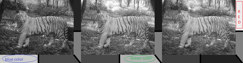
If you observe the Blue pixel image (left side), the parts of the image with blue color appear more bright and other colors similarly for Green and Red. To differentiate colors clearly I have added color borders to the original image.
- Image filtering & Blur
Gaussian blur:
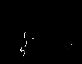
Preparing images before performing various operations is essential for accurate results. When image processing operations like edge detection, contour detection is performed noise present in an image has great impact on the outcome., before applying these algorithms on images should be processed to reduce the noise. Various noise reduction operations on images are Blurring, Erosion and Dilation.
import numpy as np
import cv2

img_data = cv2.imread("C:/Users/admin/Desktop/filter.png",1)

blur_data = cv2.GaussianBlur(img_data,(5,5),0)

cv2.imshow ("Original",img_data)

cv2.imshow ("Blur",blur_data)

cv2.waitKey(0)
cv2.destroyAllWindows()
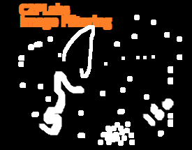
OpenCV has a GaussianBlur function to perform Gaussian blur image filtering. In the above code snippet, This function takes three arguments, first one is an image array, the second argument is kernel size (height, width), height and width should be odd numbers, the third parameter is cv.BORDER_CONSTANT = 0. The resulted output image is as shown below.
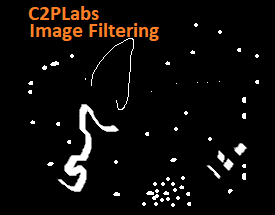
Original Image

Erosion & Dilation:
Erosion converts more white pixel into black pixels. Erosion converts pixel to value 1 if any one of the pixels in the kernel area is one. Whereas Dilation converts more black pixels into white pixels. Dilation converts pixel to value 1 only if each pixel within the kernel region is one.
kernel = np.ones((5,5),np.uint8)

erosion_img = cv2.erode(img_data,kernel,iterations = 1)
cv2.imshow("Erosion",erosion_img)

dilation_img = cv2.dilate(img_data,kernel,iterations = 1)
cv2.imshow("Dilation",dilation_img )